Transformer-Based Authorship Verification Research
Executive Summary Video
Historical Context
This research tackles a longstanding historical question concerning love letters attributed to Confederate General George E. Pickett, published posthumously by his wife LaSalle Corbell Pickett. As a prolific author with no other verified works by the General available, the letters' authenticity has been debated by historians. This presents an ideal case for authorship verification (AV) - determining if two texts share the same author.
Architecture & Implementation
 flowchart TD
     subgraph "(B) SBERT Training"
         lilat["LILAtrain"] --> batch1
         batch1["
$$B = \{(c_{\text{a}}, c_{\text{o}})_i\}_{i=1}^{\text{batch\_size}}$$
"]  --> ca1["$$C_{\text{a},i}$$"]
         batch1 --> ca2["$$C_{\text{o},i}$$"]
         ca1 --> bert1[SBERT]
         ca2 --> bert2[SBERT]
         bert1 --> pool1[Mean Pooling]
         bert2 --> pool2[Mean Pooling]
         pool1 --> ea1["$$E_{\text{a},i}$$"]
         pool2 --> eo1["$$E_{\text{o},i}$$"]
         ea1 --> contrastive[Contrastive Loss]
         eo1 --> contrastive
     end

     subgraph "(A) SBERT at Inference"
         lilai["LILAinfer"] --> batch2
         batch2["
$$B = \{(c_{\text{a}}, c_{\text{o}})_i\}_{i=1}^{\text{batch\_size}}$$
"]  --> ca3["$$C_{\text{a},i}$$"]
         batch2 --> ca4["$$C_{\text{o},i}$$"]
         ca3 --> bert3[SBERT]
         ca4 --> bert4[SBERT]
         bert3 --> pool3[Mean Pooling]
         bert4 --> pool4[Mean Pooling]
         pool3 --> ea2["$$E_{\text{a},i}$$"]
         pool4 --> eo2["$$E_{\text{o},i}$$"]
         ea2 --> cos["Cosine Similarity"]
         eo2 --> cos
         cos --> rescale["Rescaling"]
         rescale --> sim["Similarity Score [0, 1]"]
     end
     style contrastive fill:#9999ff
     style contrastive color:#000000
     style cos fill:#ff9999
     style cos color:#000000
     style rescale fill:#ff9999
     style rescale color:#000000
     style sim fill:#ff9999
     style sim color:#000000
     style lilat fill:#999999
     style lilat color:#000000
     style lilai fill:#999999
     style lilai color:#000000
Modified Contrastive Loss Implementation
Building on Hadsell, Chopra, and LeCun's foundational work (2006), implemented a modified contrastive loss function that allows for more nuanced control over embedding space distances. The implementation uses separate margin parameters for same-author and different-author pairs, enabling finer control over the model's discriminative behavior.
class ModifiedContrastiveLoss(nn.Module):
    def forward(self, anchor, other, labels):
        # Calculate cosine similarity and rescale to [0,1]
        similarities = (F.cosine_similarity(anchor, other) + 1) / 2

        # Modified loss with separate margins for same/different pairs
        same_author_loss = labels.float() * \
            F.relu(self.margin_s - similarities).pow(2)
        diff_author_loss = (1 - labels).float() * \
            F.relu(similarities - self.margin_d).pow(2)

        # Balance contribution of positive and negative pairs
        losses = 0.5 * (same_author_loss + diff_author_loss)
return losses.mean()Dataset Construction & Preprocessing
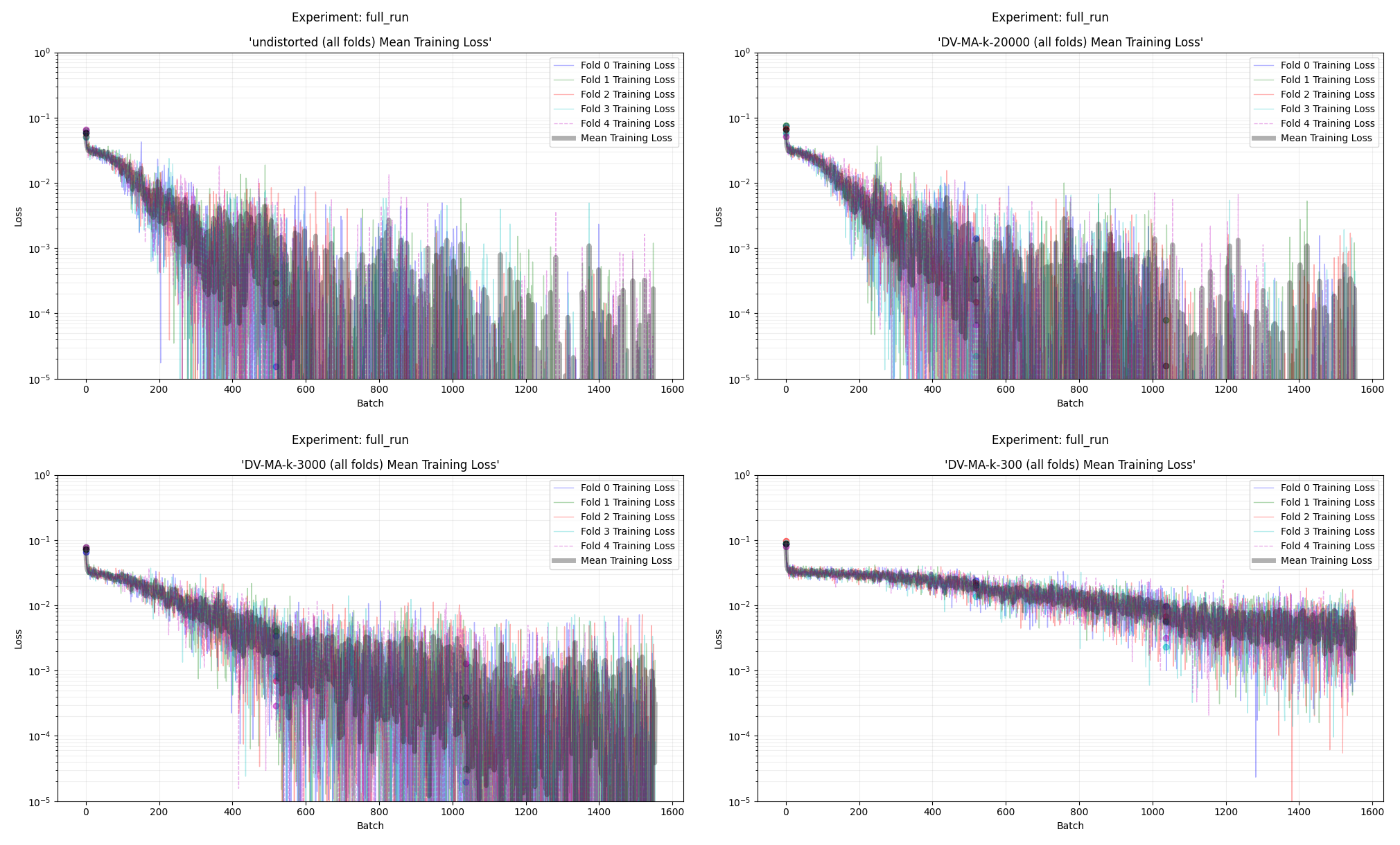
Developed LILA (Love letters, Imposters, LaSalle Augmented), a carefully balanced dataset with:
- 278,917 words of known authorial work
- 627,937 words of stylistically matched "imposters"
- Rigorous genre balancing within 10% target ratios
- Four distorted views using Stamatatos' text distortion
flowchart LR
    subgraph Disk["On-Disk Preprocessing"]
        style Disk fill:#e6f3ff,stroke:#333

        %% A -> B (subgraph) -> C
        A[("Raw Text Files")] --> B

        %% Turn B into a subgraph named "Text Normalization"
        subgraph B["Text Normalization"]
            D[Lowercase] --> E[Collapse Whitespace] --> F[Strip Special Characters]
        end

        B --> C{"Distorted View Generation"}

        C --> |"$$k_{view} = len(W_{LILA})$$"|G1[("Undistorted View")]
        C --> |"$$k_{view} = 20000$$"|G2[("Lightly Distorted")]
        C --> |"$$k_{view} = 3000$$"|G3[("Moderately Distorted")]
        C --> |"$$k_{view} = 300$$"|G4[("Heavily Distorted")]
    end

    subgraph LILA["LILADataset"]
        style LILA fill:#ffe6e6,stroke:#333
        G1 & G2 & G3 & G4 --> H[["Tokenization"]]
        H --> I[["Fixed-Length Chunking"]]
        I --> t["Generate K-Fold Train/Val Pairs"]
        I --> i["Generate Inference Pairs"]
    end

    classDef storage fill:#ff9,stroke:#333
    classDef process fill:#fff,stroke:#333
    classDef decision fill:#9cf,stroke:#333

    class A,G1,G2,G3,G4 storage
    class B,D,E,F process
    class C decision
Text Distortion Implementation
def dv_ma(text, W_k):
    """
    Replace words not in W_k (k most frequent words) with
    asterisk strings of equal length.
    """
    words = text.split()
    for i, word in enumerate(words):
        if (word.lower() in W_k):
            continue
        else:
            words[i] = re.sub(r'[^\d]', '*', word)
            words[i] = re.sub(r'[\d]', '#', words[i])
    return ' '.join(words)
Results & Analysis

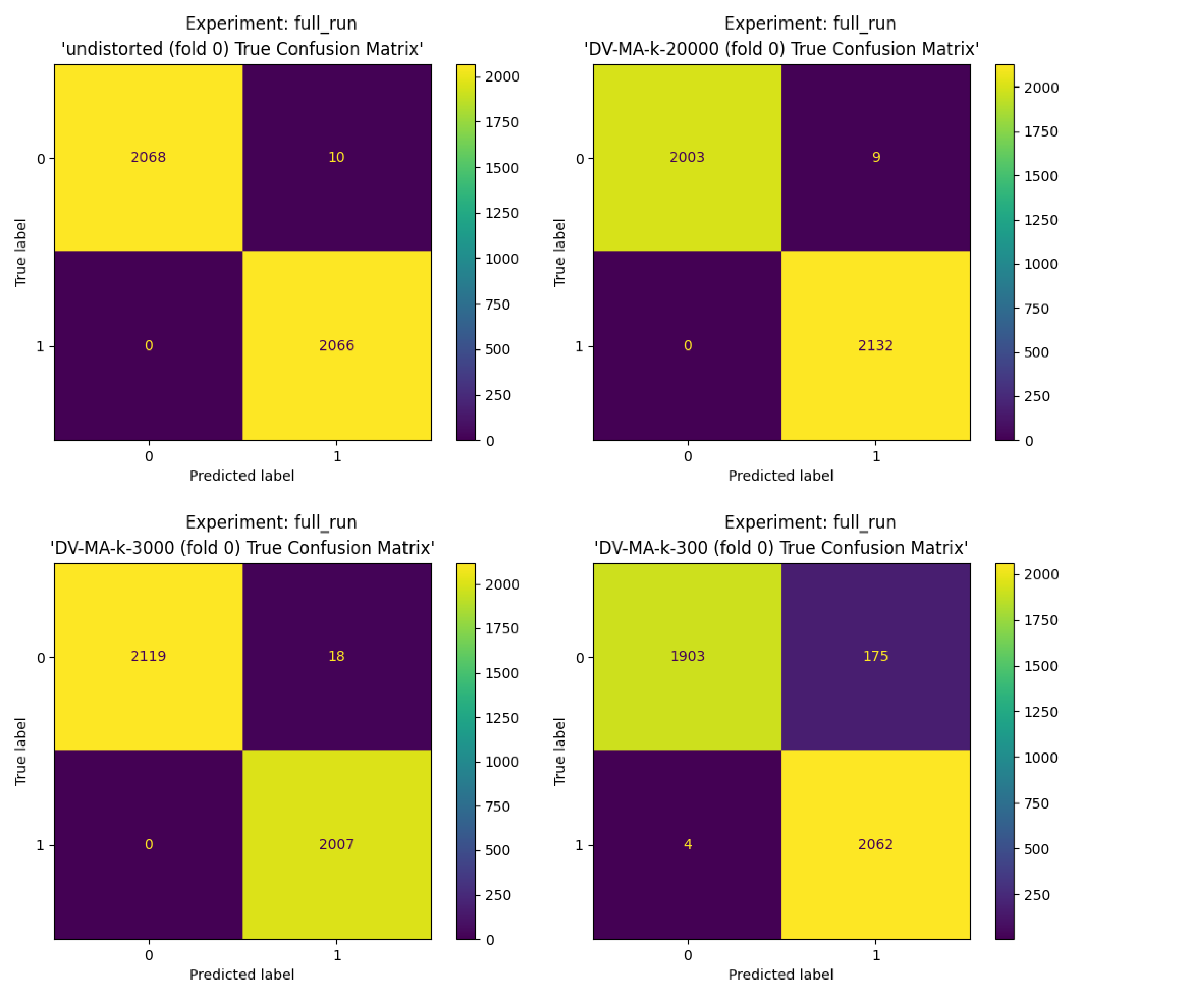
| View | AUC | C@1 | F1 | F0.5u |
|---|---|---|---|---|
| Undistorted | 1.000 ± 0.000 | 0.998 ± 0.003 | 0.998 ± 0.003 | 0.996 ± 0.005 |
| k=20,000 | 1.000 ± 0.000 | 0.996 ± 0.007 | 0.996 ± 0.006 | 0.992 ± 0.012 |
| k=3,000 | 1.000 ± 0.000 | 0.994 ± 0.003 | 0.994 ± 0.003 | 0.990 ± 0.006 |
| k=300 | 0.991 ± 0.001 | 0.964 ± 0.008 | 0.966 ± 0.007 | 0.943 ± 0.010 |
External Validation on VALLA Dataset
To validate the model's generalizability, I evaluated performance on the PAN20 sub-split of the VALLA benchmark, a comprehensive AV benchmark introduced by Tyo et al. (2022). My implementation achieved competitive results against PAN 2020 shared task participants:
| Model | Overall Score | Training Data |
|---|---|---|
| PAN20 Winner (Boenninghoff et al.) | 0.897 | PAN20-small |
| Our Implementation (30 epochs) | 0.801 | VALLA (more challenging) |
| PAN20 Baseline | 0.747 | PAN20-large |
Inference Results on the Love Letters
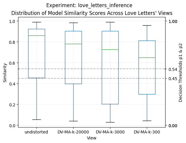
The model's analysis of the letters shows a consistent and strong pattern of attribution to LaSalle's authorship across all distortion views:
| Distorted View | Mean Similarity | Same-Author | Different-Author | Undecided |
|---|---|---|---|---|
| Undistorted | 0.709 ± 0.298 | 74.4% | 24.8% | 0.9% |
| k=20,000 | 0.661 ± 0.296 | 68.2% | 27.6% | 4.2% |
| k=3,000 | 0.598 ± 0.334 | 60.1% | 34.7% | 5.1% |
| k=300 | 0.564 ± 0.272 | 57.8% | 37.5% | 4.7% |

Technical Infrastructure
- AWS EC2 g5.xlarge deployment (4 vCPUs, 16GB RAM, NVIDIA A10G GPU)
- PyTorch with HuggingFace Transformers
- Custom dataset class handling 10M+ words
- Gradient accumulation for memory efficiency
- K-Folds cross-validation with balanced splits
