The Queen's Gambit: A Machine Learning Analysis of the Chess Community's Attitude After the Hit Netflix Show 
Did The Queen's Gambit Change the Chess Community's Attitude toward Women?
An analysis of sentiment in posts regarding women from chess.com before and after the airing of the hit Netflix show
Most who have spent even a small amount of time in the world of chess know that it can be a sexist space. It is a community containing many respected intellectual elites, many of whom are prone to endorsing discriminatory ideas, such as Nigel Short saying men are 'hardwired' to be better chess players[1]. Interestingly though, arguably the most significant cultural event to occur in the chess space since World Champion Garry Kasparov was defeated by IBM's Deep Blue Computer in 1997, was the airing (and subsequent ascent to Netflix's most-watched scripted series[2]) of the female lead and centered chess drama The Queen's Gambit.
I wanted to know whether the advent of this show, which does not shy away from showing the misogyny inherent in chess, has affected any shift in the relationship of the chess community at large towards women in the royal game.
How could I begin to investigate this idea?
My strategy
I spent an afternoon considering how to go about researching this question, and here are the steps I came up with:
- Retrieving the data: I would find an online community as close to representative of the chess community at large as I could and retrieve said community's posts, comments, or other sorts of data over an appropriate span of time so that I could see any trends related to the debut of The Queen's Gambit
- Cleaning the data: I would then need to clean my data by removing empty, erroneous, aberrant, or otherwise problematic data
- Tokenizing the data: Next, I would have to 'tokenize' my data to convert strings to more easily usable data structures for my algorithms
- Normalizing the data: Then, I would have to normalize my data to remove data not useful to a computer and bring the data remaining down to its basic forms
- Finding female words: Now, I would reduce my data set down to only those posts which refer to women in some way
- Performing Sentiment Analysis: I would now need to run sentiment analysis on my data and store my results
- Removing outliers: At this point, I would need to find outliers in the sentiment scores and deal with the associated data point appropriately
- Plotting the data: Penultimately, I would have to plot my results along with any descriptive or summative plots (such as lines of best fit)
- Conclusion: Finally, I would need to draw any conclusions from my data, if any were to be inferred, and talk about the project and findings in a broader way, including issues and takeaways
I also looked around to see if this question had already been addressed and could not find any such study. A couple of noteworthy studies used sentiment analysis in the context of the chess community's reaction to The Queen's Gambit (which I cite at the end of this paper). However, none of them focused on the question of sexism particularly.
I planned to study sentiment relating to women within the chess community, not sentiment relating to the series.
I had outlined a strategy for myself, and it was now time to start on step one.
Retrieving the data
Firstly, and most fundamentally, I needed data. I decided to use the General Forum[3] of the website Chess.com. I chose this because chess.com has the largest userbase currently on any chess website, and therefore I expect it to be the most representative of the community. I also considered using lichess.org forums as well as the subreddit r/chess. I chose not to use lichess.org because its userbase is far smaller than that of chess.com, and I chose against r/chess since there is no easy way to scrape posts chronologically from Reddit.
I needed a significant window of time to collect data so that I could compare before and after the show aired. I chose to gather data using the airing of the show (October 23rd, 2020) as a pivot, collecting posts from that moment to the present (June 20th, 2021 at the time) and before that moment back the same amount of time (roughly March 12th, 2020).
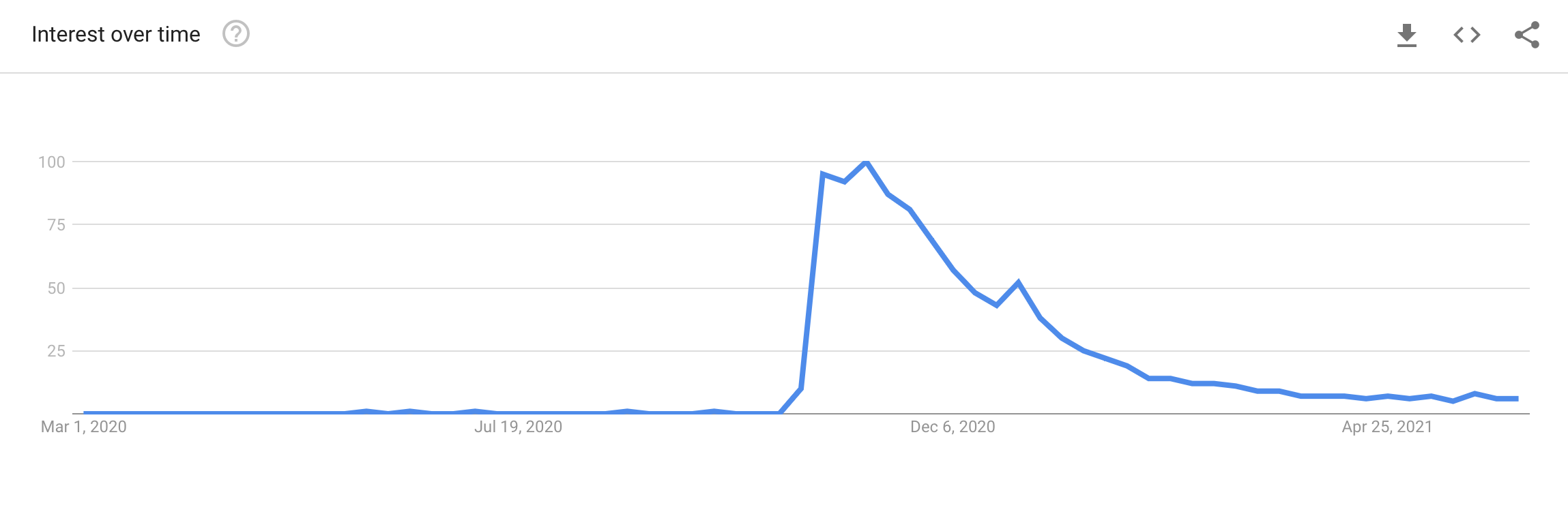
Google Trends[4] unsurprisingly shows a clear spike in the search term "Queen's Gambit" at precisely the airing of the hit show, and a gradual fall off to slightly above its previous baseline thereafter.
This data seemed promising. So now it was time actually to retrieve the data. To accomplish the data retrieval part of this study, I would need the requests and time packages for getting the raw pages from the chess.com forums, BeautifulSoup to navigate that raw data, and NumPy, pandas, DateTime, and CSV to process and save it.
I also went ahead and saved the starting page from which my algorithm would begin its scraping of the chess.com forum (a seed as it were) and the date at which I wanted to stop retrieving data.
# Import requisite packages
# setup global variables
# and read in data
import requests
import csv
import time
from bs4 import BeautifulSoup
from datetime import datetime
import pandas as pd
import numpy as np
# web address for the "General Chess Discussion" forum on Chess.com
first_page_url = "https://www.chess.com/forum/category/general"
# date representing the farthest back in the forum you wish to post
# not precise, might pull in a few posts older than defined stop date
stop_date = datetime(2020, 3, 12)
I would need to retrieve pages from chess.com more than once, as
the forum is structured as many pages of links to threads. So I
constructed a function for obtaining the BeautifulSoup
representation of a page, given its URL as an input, as seen
below in the function get_soup(). (modified from code provided by Prof. McGrath in class[5])
# get_soup() is modified from code shown in a lecture by Sean McGrath @ https://www.coursera.org/learn/uol-cm2015-programming-with-data/lecture/kWE1l/5-05-introduction-to-web-scraping
def get_soup(URL, jar=None, print_output=False):
    if print_output:
        print("scraping {}".format(URL))
    request_headers = {
        "update-insecure-requests": "1",
        "user-agent": "Mozilla/5.0 (Windows NT 6.1; Win64; x64; rv:47.0) Gecko/2010 0101 Firefox/47.0",
        "accept": "*/*",
        "accept-encoding": "gzip, deflate, br",
        "accept-language": "en-US,en;q=0.8"
    }
    if jar:
        r = requests.get(URL, cookies=jar, headers=request_headers)
    else:
        r = requests.get(URL, headers=request_headers)
        jar = requests.cookies.RequestsCookieJar()
    data = r.text
    soup = BeautifulSoup(data, "html.parser")
    return soup, jar
Since the main view from the forum is that of a page of links to
posts, each only containing a small preview of the post, I would
need to take this in two stages. First, obtain all the links
within my window of time, then obtain all posts and comments
from the collected links. As these links are spread over many
pages, I decided to create a general function that could receive
the BeautifulSoup representation of the page and return the
links contained within. This I did with
get_page_post_links() shown below. Of note is the
returned value earliest_post_data, which acts as a
control flag. With this, my main routine can compare the data of
the earliest post found on the returned page against the global
stop_date to determine if it should continue.
# function for retrieving all the relevant posts on a particular page
def get_page_post_links(soup):
    # make a container to hold and work with collected posts
    # and keep track of the current date
    post_links = []
    earliest_post_date = None
    # get post thumbnails with bs4
    post_preview_elements = soup.find_all("tr", class_="forums-category-thread-row")
    # extract links and dates from previews
    for post_preview_element in post_preview_elements:
        post_links.append(
            post_preview_element.find_all(
                "a",
                class_="forums-category-thread-title"
            )[0]['href']
        )
        latest_elem = post_preview_element.find_all("div", class_="forums-category-thread-latest-row")
        time_elem = latest_elem[1].find_all("span")
        earliest_post_date = time_elem[0]['title']
    earliest_post_date = datetime.strptime(earliest_post_date, "%b %d, %Y, %I:%M:%S %p")
    return post_links, earliest_post_date
Now I was ready to write a function that could call the previous
two iteratively to walk through each page in the forum and
combine all the links into one collection for individual
scraping. It's worth pointing out here that I included some
print() statements here, as well as within
get_soup() so that I could keep an eye on things as
they processed. It's also important to note that I used the
sleep() function from the time package
(line 21 of get_posts_over_time_period() and line 7
of get_data_from_posts()) to force a pause between
each call to chess.com's servers. The purpose was both to
prevent me from getting blocked from chess.com and not to
overburden their own servers and cause any problems for them or
their users.
# function for paginating through the forum and retrieving all posts submitted
# after a user-defined start date (stop_date)
def get_posts_over_time_period(url, stop_date):
    # assign the control variable the default time of now
    # as we know this will be later than the input stop_data
    earliest_post_date_on_page = datetime.now()
    # container for post links
    all_post_links = []
    soup, jar = None, None
    num_collected = 0
    # while the earliest found data on the page is still greater
    # then our desired stop point, continue collecting all post links
    while (earliest_post_date_on_page > stop_date):
        # print output periodically for user monitoring
        print_output = num_collected % 2000 == 0
        if print_output:
            print(
                "{} > {}: proceeding".format(
                    earliest_post_date_on_page.strftime("%b %d, %Y, %I:%M:%S %p"),
                    stop_date.strftime("%b %d, %Y, %I:%M:%S %p")
                )
            )
        # if first call, collect cookies, otherwise include collected
        # cookies, find link to next page, and implement wait to avoid
        # being flagged as a bot and reduce strain on chess.com's servers
        if (soup == None):
            soup, jar = get_soup(url, None, print_output)
        else:
            link_to_next_page = soup.find("a", class_="pagination-next")['href']
            time.sleep(2)
            soup, jar = get_soup(link_to_next_page, jar, print_output)
        # get all links to posts on page
        post_links, earliest_post_date_on_page = get_page_post_links(soup)
        # add to container
        all_post_links.extend(post_links)
        # updated our tracker for output printing
        num_added = len(post_links)
        num_collected += num_added
        if print_output:
            print("added {} posts".format(num_added))
            print("{} collected".format(num_collected))
    return pd.DataFrame(all_post_links, index=range(len(all_post_links)), columns=['link'])

post_links_df = get_posts_over_time_period(first_page_url, stop_date)
post_links_df.to_csv("data/forum_page_links.csv")
Jun 19, 2021, 05:54:21 PM > Mar 12, 2020, 12:00:00 AM: proceeding
scraping https://www.chess.com/forum/category/general
added 20 posts
20 collected
May 25, 2021, 05:13:05 AM > Mar 12, 2020, 12:00:00 AM: proceeding
scraping https://www.chess.com/forum/category/general?page=101
added 20 posts
2020 collected
May 02, 2021, 03:08:11 AM > Mar 12, 2020, 12:00:00 AM: proceeding
scraping https://www.chess.com/forum/category/general?page=201
added 20 posts
4020 collected
Apr 09, 2021, 03:35:35 PM > Mar 12, 2020, 12:00:00 AM: proceeding
scraping https://www.chess.com/forum/category/general?page=301
added 20 posts
6020 collected
Mar 12, 2021, 01:19:36 PM > Mar 12, 2020, 12:00:00 AM: proceeding
scraping https://www.chess.com/forum/category/general?page=401
added 20 posts
8020 collected
Feb 15, 2021, 04:49:00 PM > Mar 12, 2020, 12:00:00 AM: proceeding
scraping https://www.chess.com/forum/category/general?page=501
added 20 posts
10020 collected
Jan 20, 2021, 10:45:19 AM > Mar 12, 2020, 12:00:00 AM: proceeding
scraping https://www.chess.com/forum/category/general?page=601
added 20 posts
12020 collected
Dec 18, 2020, 05:33:41 PM > Mar 12, 2020, 12:00:00 AM: proceeding
scraping https://www.chess.com/forum/category/general?page=701
added 20 posts
14020 collected
Nov 13, 2020, 06:39:45 PM > Mar 12, 2020, 12:00:00 AM: proceeding
scraping https://www.chess.com/forum/category/general?page=801
added 20 posts
16020 collected
Oct 03, 2020, 06:35:52 PM > Mar 12, 2020, 12:00:00 AM: proceeding
scraping https://www.chess.com/forum/category/general?page=901
added 20 posts
18020 collected
Aug 20, 2020, 12:26:21 AM > Mar 12, 2020, 12:00:00 AM: proceeding
scraping https://www.chess.com/forum/category/general?page=1001
added 20 posts
20020 collected
Jul 03, 2020, 04:52:57 AM > Mar 12, 2020, 12:00:00 AM: proceeding
scraping https://www.chess.com/forum/category/general?page=1101
added 20 posts
22020 collected
May 17, 2020, 12:05:01 PM > Mar 12, 2020, 12:00:00 AM: proceeding
scraping https://www.chess.com/forum/category/general?page=1201
added 20 posts
24020 collected
Mar 25, 2020, 01:40:22 AM > Mar 12, 2020, 12:00:00 AM: proceeding
scraping https://www.chess.com/forum/category/general?page=1301
added 20 posts
26020 collected
Now I had links to every post within my chosen window of time saved to a CSV file on my machine.
post_links_df = pd.read_csv("data/forum_page_links.csv", index_col=0)
print("I've collected {} posts!".format(len(post_links_df)))
I've collected 26380 posts!
I had collected over 25,000 posts - and that's not counting comments on each of those posts. I felt like I had a fairly large dataset. But now, I actually needed to get the content of these posts and their comments. The links alone were of no help to me.
So I wrote the function get_data_from_posts(),
which would take in my collection of post links and grab the
BeautifulSoup representation of each post page and pluck out the
relevant content (text content and time stamp for both the
original post and all comments on it).
# function for getting links to full posts
def get_data_from_posts(links):
    # make a container to hold and work with collected data
    rows = []
    total = len(links)
    for i, link in enumerate(links[:]['link']):
        time.sleep(2)
        print_output = len(rows) % 2000 == 0
        soup, _ = get_soup(link, None, print_output)
        if print_output:
            print(
                "{}/{}".format(
                    i + 1,
                    total
                )
            )
        # grab all comments
        comments = soup.find_all('div', class_="comment-post-component")
        for comment in comments:
            try:
                text = comment.find('p').text
            except:
                text = ""
            try:
                # try to obtain a timestamp
                timestamp_string = comment.find('span', class_="comment-post-actions-time").find('span')['title']
                timestamp = datetime.strptime(timestamp_string, "%b %d, %Y, %I:%M:%S %p")
            except:
                # if cannot, use np.nan
                timestamp = np.nan
            rows.append({
                "text": text,
                "timestamp": timestamp
            })
    post_data = pd.DataFrame(rows, index = range(len(rows)))
    return post_data

data = get_data_from_posts(post_links_df)
data.to_csv("data/data.csv")
scraping https://www.chess.com/forum/view/general/how-to-contact-support
1/26380
scraping https://www.chess.com/forum/view/general/why-are-people-being-mean-to-me-lately
712/26380
scraping https://www.chess.com/forum/view/general/prove-it
2557/26380
scraping https://www.chess.com/forum/view/general/flagging-is-it-unethical-or-part-of-the-game
2806/26380
scraping https://www.chess.com/forum/view/general/https-rumble-com-vfv1p3-its-back-to-the-board-for-chess-grandmasters-html
5103/26380
scraping https://www.chess.com/forum/view/general/chess-survey-mental-speed-study
6704/26380
scraping https://www.chess.com/forum/view/general/is-chess-finally-dead
7562/26380
scraping https://www.chess.com/forum/view/general/why-did-bobby-fischer-quit-chess
8135/26380
scraping https://www.chess.com/forum/view/general/bot-ratings-and-improvements
10280/26380
scraping https://www.chess.com/forum/view/general/wait-what-1
14065/26380
scraping https://www.chess.com/forum/view/general/disabled-chess-players-out-there
15583/26380
scraping https://www.chess.com/forum/view/general/what-do-you-guys-think-about-the-wijk-aan-zee-2013-tournament
16187/26380
scraping https://www.chess.com/forum/view/general/wrong-threefold-repetition
20522/26380
scraping https://www.chess.com/forum/view/general/can-we-see-are-pending-requests
20844/26380
scraping https://www.chess.com/forum/view/general/probleem-onvoldoende-materiaal
25044/26380
This function took almost 24 hours to iterate through my entire collection of post links; however, I ended up with 175,817 individual posts/comments!
data = pd.read_csv("data/data.csv", index_col=0)
print("I've collected {} data points!".format(len(data)))
I've collected 175817 data points!
Let's take a peek at this data.
data[400:440]
| text | timestamp | |
|---|---|---|
| 400 | | 2021-06-19 05:40:54 |
| 401 | we need to contact chess.com staff and issue a... | 2021-06-19 07:32:51 |
| 402 | Its so pathetic that they don't tell you you a... | 2021-06-19 07:40:06 |
| 403 | A single Mod dictator rules over LC . Break To... | 2021-06-19 07:42:12 |
| 404 | A single Mod dictator rules over LC . Break To... | 2021-06-19 07:46:19 |
| 405 | I realize I’m not the sharpest tool in the she... | 2021-06-19 08:12:17 |
| 406 | Its so pathetic that they don't tell you you a... | 2021-06-19 08:14:01 |
| 407 | we can be shadow ban brothers till the end of ... | 2021-06-19 08:14:15 |
| 408 | hhhello | 2021-06-19 08:14:25 |
| 409 | i got shadow banned | 2021-06-19 08:20:49 |
| 410 | we are all shadow ban brothers then | 2021-06-19 08:21:14 |
| 411 | we will rise up | 2021-06-19 08:21:20 |
| 412 | pray to our leder erik | 2021-06-19 08:21:27 |
| 413 | and when the time comes we will storm the lich... | 2021-06-19 08:21:48 |
| 414 | THE CULT OF ERIK | 2021-06-19 08:21:56 |
| 415 | I have seen a lot of advice for beginners that... | 2021-05-30 09:15:00 |
| 416 | Reasons i dont castle, if the queens come off ... | 2021-05-30 09:42:45 |
| 417 | There is no "one size fits all" answer. Castle... | 2021-05-30 09:57:57 |
| 418 | If you know your openings then you know when i... | 2021-05-30 10:12:57 |
| 419 | When u play the bongcloud | 2021-05-30 10:20:10 |
| 420 | To add a little nuance I take a different appr... | 2021-05-30 10:57:56 |
| 421 | Castling as quickly as possible leads to a saf... | 2021-05-30 11:57:39 |
| 422 | I found this series by Gotham chess on prevent... | 2021-06-01 01:44:10 |
| 423 | When the center is closed, sometimes it's bett... | 2021-06-01 02:00:12 |
| 424 | Castling is nearly always good. O-O is like 3 ... | 2021-06-01 02:05:54 |
| 425 | I have been looking through GM games. It is ra... | 2021-06-01 02:21:05 |
| 426 | You probably shouldn't castle when there is a ... | 2021-06-01 03:35:07 |
| 427 | @KevinOSh very perceptive! | 2021-06-01 03:48:24 |
| 428 | Just watched this video covering the game Sieg... | 2021-06-02 03:51:28 |
| 429 | I usually castle when possible, but i suck at ... | 2021-06-02 04:05:48 |
| 430 | When the centre is closed you don't need to ru... | 2021-06-02 05:44:07 |
| 431 | I usually castle when possible, but i suck at ... | 2021-06-02 07:46:32 |
| 432 | dont castle if: | 2021-06-02 07:49:05 |
| 433 | Reasons i dont castle, if the queens come off ... | 2021-06-02 08:02:36 |
| 434 | ‘Good players seldom castle’ | 2021-06-02 08:09:32 |
| 435 | How do you do this and make this in your descr... | 2021-06-10 07:38:24 |
| 436 | hi | 2021-06-10 07:57:27 |
| 437 | hi | 2021-06-10 07:57:43 |
| 438 | NaN | 2021-06-10 07:58:06 |
| 439 | how do you do that? | 2021-06-10 07:58:35 |
It looks good, but I already see two problems. We have an empty post, or perhaps just whitespace, at index 400 and an NaN value at index 438. It's time to do some cleanup.
print(data[data.eq('2021-06-19 05:40:54').any(1)])
print(data[data.eq('2021-06-10 07:58:06').any(1)])
text timestamp
400 2021-06-19 05:40:54
text timestamp
438 NaN 2021-06-10 07:58:06
Cleaning the data
Now that I had my data, I needed to clean it up and get it ready for analysis. To help me with this, I again used the NumPy, DateTime, and pandas packages.
I also still had use for the stop_date variable, as
I'll explain shortly.
# Import requisite packages
# setup global variables
# and read in data
from datetime import datetime
import pandas as pd
import numpy as np
# setup earliest date of interest in this study
stop_date = datetime(2020, 3, 12)
# read in data
data = pd.read_csv("data/data.csv", index_col=0)
First, I converted all the datetime strings from my CSV back to
datetime objects with the pandas function
to_datetime().
# convert timestamp strings to datetime objects
data['timestamp'] = pd.to_datetime(data['timestamp'], format="%Y-%m-%d %H:%M:%S")
Next, I used a handy
regular expression provided by patricksurry[6] at StackOverflow to substitute all empty strings
and comments that were completely white space, for
np.nan.
# code modified from https://stackoverflow.com/a/21942746
# replace field that's entirely white space (or empty) with NaN
cleaned_data_1 = data.replace(r'^\s*$', np.nan, regex=True).copy()
With the help of a line of code from yulGM[7], again at StackOverflow, I masked out all comments which were only one character long (these do not contain enough meaning for sentiment analysis to be viable).
# code modified from https://stackoverflow.com/a/64837795
# remove all rows where text is 1 character in length
cleaned_data_2 = cleaned_data_1[np.where((cleaned_data_1['text'].str.len() == 1), False, True)].copy()
Next, I removed all comments where the text or the timestamp
were "empty," which, because of the processes above, were now
all flagged by np.nan.
# remove missing data
cleaned_data_3 = cleaned_data_2.dropna().copy()
I was almost there, but I had one cleaning chore left. Because the format of the chess.com forums is not quite as simple as I may have implied above, I likely still had comments from outside of my desired time frame. Rather than simply showing the most recent post first and subsequent posts in a descending fashion, chess.com forums show the most recently updated post first followed by less recently updated posts in a descending fashion. "Updated" here means brand new posts or posts which have received a new comment. This meant that I had data outside of my chosen window of time. For example: if a post from 2019 had just had its first new post in over a year yesterday, I would have grabbed it up, along with any of its old comments, since it was updated within my time frame!
The first step to removing these wayward posts was to sort my dataset by the time of the posts.
# sort data by timestamp
cleaned_data_4 = cleaned_data_3.sort_values('timestamp', 0).copy()
Using a similar method to that which I used to remove one
character long posts above, I masked out all posts that had a
timestamp earlier than my earliest date of interest (this is why
I still needed stop_date above).
# remove all data from outside our chosen time window
cleaned_data_5 = cleaned_data_4[np.where((cleaned_data_4['timestamp'] < stop_date), False, True)].copy()
cleaned_data_5.to_csv("data/data_cleaned.csv")
Great! After all this cleaning, let's see how many posts I'm left with.
data_cleaned = pd.read_csv("data/data_cleaned.csv", index_col=0)
print("I now have {} data points!".format(len(data_cleaned)))
I now have 123032 data points!
And let's take a look at my cleaned-up dataset now.
print(data_cleaned[data_cleaned.eq('2021-06-19 05:40:54').any(1)])
print(data_cleaned[data_cleaned.eq('2021-06-10 07:58:06').any(1)])
Empty DataFrame
Columns: [text, timestamp]
Index: []
Empty DataFrame
Columns: [text, timestamp]
Index: []
The problematic posts pointed out above are gone, and the timestamp column is nicely sorted starting early on our first day of interest, as we should expect.
The data was now ready to be prepared for sentiment analysis!
Tokenizing the data
To be analyzed and prepared for sentiment analysis, I needed to discretize my data into 'tokens' - individual chunks of syntactic meaning, typically as words, punctuation, symbols, emojis, links, and other things.
To do this, I would, as always, need my good friends datetime, pandas, and NumPy, but also a new package called nltk. (natural language toolkit)
# Import requisite packages
# and read in data
from datetime import datetime
import pandas as pd
import numpy as np
import nltk
# read in data
# NOTE: you will need to run the cells from the "Cleaning the data" section
# above in order to read in this data.
# If you do not, this cell the the following cells will throw errors
# when you attempt to run them.
clean_data = pd.read_csv("data/data_cleaned.csv", index_col=0)
Using an anonymous function based off of
Carlos Mougan's code[8], this time at StackExchange, I applied nltk's
word_tokenize() function row by row over my dataset
outputting to an array which I then appended as a new column,
"tokens," to my dataset.
# code modified from https://datascience.stackexchange.com/a/68002
tokens = clean_data.apply(lambda row: nltk.word_tokenize(row.iloc[0]), axis=1).copy()
clean_data['tokens'] = tokens.copy()
Let's see our data after this.
clean_data.head()
| text | timestamp | tokens | |
|---|---|---|---|
| 175718 | How much is average fees for local chess tourn... | 2020-03-12 00:03:31 | [How, much, is, average, fees, for, local, che... |
| 175726 | A good looking chess piece. | 2020-03-12 00:25:31 | [A, good, looking, chess, piece, .] |
| 175728 | Nice! | 2020-03-12 00:26:44 | [Nice, !] |
| 175729 | Which one? | 2020-03-12 00:27:14 | [Which, one, ?] |
| 175730 | Let’s play! | 2020-03-12 00:27:28 | [Let, ’, s, play, !] |
It looks like I expected it to look; however, it had two problems. It's very redundant and memory inefficient since 'text' and 'tokens' are identical in every way except the data structure in which they're held. It's also awkward to have a whole array stored as a cell within another array-like data structure. We'll fix this by storing only the tokens column and flattening each token into its own row.
To accomplish the latter fix, I used the pandas function
explode(), which does exactly what I was looking
for - giving each token its own row, which takes its index from
the index of its originating row. I fixed the former issue by
copying only the 'tokens' and 'timestamp' columns into a new
DataFrame.
# make a row for each token with a copy of data from originating row
data_exploded = clean_data.explode('tokens')
# make a new dataframe of our data flattened out
# tokens are indexed by timestamp and sub-indexed by order of occurrence within a post
data_tokenized = pd.DataFrame(data_exploded['tokens'].to_list(),
                              index=[
                                  data_exploded['timestamp'],
                                  [item for sublist in clean_data['tokens'] for item in range(len(sublist))]
                              ],
                              columns=['tokens'])
data_tokenized.to_csv("data/data_tokenized.csv")
I also introduced a second index at this point for ease of human readability. This was a simple index that indicates the 'position' of a token within a comment. This takes us from more common data structures to what pandas calls a multi-index dataframe, i.e., a hierarchical data representation.
Let's see what I mean.
data_tokenized.iloc[46:63]
| tokens | ||
|---|---|---|
| timestamp | ||
| 2020-03-12 00:27:28 | 0 | Let |
| 1 | ’ | |
| 2 | s | |
| 3 | play | |
| 4 | ! | |
| 2020-03-12 00:47:22 | 0 | Мне |
| 1 | тоже | |
| 2 | прислали | |
| 3 | ! | |
| 2020-03-12 01:05:32 | 0 | They |
| 1 | did | |
| 2 | not | |
| 3 | have | |
| 4 | the | |
| 5 | resources | |
| 6 | , | |
| 7 | engines |
As you can see, there are now groups of rows indexed by their timestamps, where their relative positions within the comments are our secondary index within the groups.
But, again, I see some problems with my data. Punctuation such as periods, while helpful for me to read and understand the pacing and connectivity of sentences, is not particularly helpful for basic sentiment analysis algorithms and introduces noise and unnecessary compute cycles. Also, one of the comments is in Russian. While non-English comments are something another study could include, it is outside this project's scope.
It was now time for me to normalize my data and eradicate these issues.
Normalizing the data
Normalizing data in the context of natural language means removing "noisy" tokens (chunks of language which do not hold enough meaning to be useful to a computer) and bring all other words down to their basic forms. (running = run, lady = woman, etc.)
To accomplish this, I was going to need some help from nltk. Along with nltk, I was still going to need NumPy, pandas, and datetime, as well as re and string.
# Import requisite packages
# setup global variables
# and read in data
from datetime import datetime
import pandas as pd
import numpy as np
import nltk
nltk.download('wordnet')
nltk.download('averaged_perceptron_tagger')
from nltk.tag import pos_tag
from nltk.stem.wordnet import WordNetLemmatizer
import re, string
from nltk.corpus import stopwords
data_to_normalize = pd.read_csv("data/data_tokenized.csv", index_col=[0, 1])
[nltk_data] Downloading package wordnet to
[nltk_data]     /Users/zacbolton/nltk_data...
[nltk_data]   Package wordnet is already up-to-date!
[nltk_data] Downloading package averaged_perceptron_tagger to
[nltk_data]     /Users/zacbolton/nltk_data...
[nltk_data]   Package averaged_perceptron_tagger is already up-to-
[nltk_data]       date!
/opt/homebrew/Caskroom/miniforge/base/lib/python3.9/site-packages/numpy/lib/arraysetops.py:583: FutureWarning: elementwise comparison failed; returning scalar instead, but in the future will perform elementwise comparison
  mask |= (ar1 == a)
With a lot of help from this article by Shaumik Daityari[9] I wrote up a function that could normalize my a post from my data.
It uses re to match and remove all tokens, which are emails or links. It also removes all tokens which match nltk's English stop words corpus or string's punctuation corpus. Finally, it stems (brings words down to their basic form) the remaining tokens using nltk's VADER (Valence Aware Dictionary and sEntiment Reasoner) sentiment analysis algorithm.
# code modified from https://www.digitalocean.com/community/tutorials/how-to-perform-sentiment-analysis-in-python-3-using-the-natural-language-toolkit-nltk
def remove_noise(tokens, stop_words = ()):

    cleaned_tokens = []

    # pos_tag does not work on every tokenized string
    # '\' seems to cause it to fail.
    # if pos_tag fails, return a flag, so the superroutine
    # can react accordingly
    try:
        tags = pos_tag(tokens)
    except:
        return False

    for token, tag in tags:
        # remove punctuation or emails
        token = re.sub('http[s]?://(?:[a-zA-Z]|[0-9]|[$-_@.&+#]|[!*\(\),]|'\
                       '(?:%[0-9a-fA-F][0-9a-fA-F]))+','', token)
        token = re.sub("(@[A-Za-z0-9_]+)","", token)

        if tag.startswith("NN"):
            pos = 'n'
        elif tag.startswith('VB'):
            pos = 'v'
        else:
            pos = 'a'

        # stem tokens
        lemmatizer = WordNetLemmatizer()
        token = lemmatizer.lemmatize(token, pos)

        # remove if empty, punctuation, or stop-word
        if len(token) > 0 and token not in string.punctuation and token.lower() not in stop_words:
            cleaned_tokens.append(token.lower())
    return cleaned_tokens
Now I just needed to run each post in my dataset through
remove_noise(). The loop below does just this and
unsurprisingly takes a few minutes to complete.
# create containers for columns and indices
time_index = []
pos_index = []
normalized_tokens = []

# loop through data by first hierarchical index (post)
# remove noise from tokens, and add to containers
for time, tokens in data_to_normalize.groupby(level=0):
    tokens = remove_noise(tokens['tokens'], stopwords.words('english'))
    if tokens == False:
        pass
    else:
        time_index.extend([time for x in range(len(tokens))])
        pos_index.extend([x for x in range(len(tokens))])
        normalized_tokens.extend(tokens)

data_normalized = pd.DataFrame({'tokens': normalized_tokens}, index=[time_index, pos_index])

data_normalized.to_csv("data/data_normalized.csv")
As usual, let's take a look at our data before moving on.
data_normalized.iloc[24:37]
| tokens | ||
|---|---|---|
| 2020-03-12 00:27:28 | 0 | let |
| 1 | ’ | |
| 2 | play | |
| 2020-03-12 00:47:22 | 0 | мне |
| 1 | тоже | |
| 2 | прислали | |
| 2020-03-12 01:05:32 | 0 | resource |
| 1 | engine | |
| 2 | internet | |
| 3 | study | |
| 4 | use | |
| 5 | write | |
| 6 | .... |
As we can see, our data retains our desired structure but has been changed quite a lot. It is now much more difficult for us to understand; however, it is much easier for a computer to read with regard to sentiment.
The Russian post is not yet gone, however the next step will remove it since it is going to pull out posts based on female pronouns and other words for women in english and no other language.
Finding female words
Now I needed to prune my dataset down to only those posts which
talk about women. To do this, I would still need pandas and
NumPy as usual. I also would need my
remove_noise() function from above along with its
nltk dependencies.
# Import requisite packages
# setup global variables
# and read in data
import pandas as pd
import numpy as np
import nltk
from nltk.tag import pos_tag
import re, string
from nltk.stem.wordnet import WordNetLemmatizer
data_normalized = pd.read_csv("data/data_normalized.csv", index_col=[0, 1])
/opt/homebrew/Caskroom/miniforge/base/lib/python3.9/site-packages/numpy/lib/arraysetops.py:583: FutureWarning: elementwise comparison failed; returning scalar instead, but in the future will perform elementwise comparison
  mask |= (ar1 == a)
Now that I had my necessary packages, I needed to define what a
'female word' was in the context of this study. Below are those
words I chose. It is worth noting that the first four "words"
listed are abbreviations for the chess titles, Woman
Grandmaster, Woman FIDE Master, Woman International, and Woman
Candidate Master. The code below takes my collection of words,
runs it through the remove_noise() function to
align it with the dataset, and then inputs that into a
set() to remove duplicates.
# Female verbiage to filter data by
female_words = set(
    remove_noise(
        [
            'wgm',
            'wfm',
            'wim',
            'wcm',
            'her',
            'hers',
            'she',
            'girl',
            'woman',
            'women',
            'girls',
            'female',
            'females',
            'lady',
            'ladies',
            'wife',
            'sister',
            'mother',
            'daughter',
            'niece',
            'girlfriend',
            "women's",
            "woman's",
            'gal',
            'dame',
            'lass',
            'chick'
        ]
    )
)
Now it was time to loop through my posts and pull out all those posts which contain at least one of the words I had identified above.
# create containers for columns and indices
time_index = []
pos_index = []
normalized_tokens = []

# again, loop through data by first hierarchical index (post)
# if it is pairwise disjoint from our set of female verbiage
# do nothing, otherwise save it to containers
for time, tokens in data_normalized.groupby(level=0):
    words = tokens.values.flat
    if (not set(words).isdisjoint(female_words)):
        # if the post contains at least one of the words in female_words, keep it
        times = [time for x in range(len(tokens))]
        time_index.extend(times)

        positions = [x for x in range(len(tokens))]
        pos_index.extend(positions)

        normalized_tokens.extend(tokens.values.flat)

posts_containing_female_words = pd.DataFrame({'tokens': normalized_tokens}, index=[time_index, pos_index])

posts_containing_female_words.to_csv("data/posts_containing_female_words.csv")
Let's again take a look at our data and see if everything looks right.
posts_containing_female_words.iloc[0:37]
| tokens | ||
|---|---|---|
| 2020-03-14 04:08:19 | 0 | take |
| 1 | mine | |
| 2 | local | |
| 3 | bar | |
| 4 | use | |
| 5 | pick | |
| 6 | chick | |
| 7 | know | |
| 8 | excited | |
| 9 | girl | |
| 10 | get | |
| 11 | find | |
| 12 | play | |
| 13 | chess | |
| 14 | ... | |
| 2020-03-19 17:01:18 | 0 | fine |
| 1 | start | |
| 2 | look | |
| 3 | game | |
| 4 | one | |
| 5 | played | |
| 6 | person | |
| 7 | also | |
| 8 | 1000s | |
| 9 | make | |
| 10 | 75 | |
| 11 | best | |
| 12 | move | |
| 13 | possible | |
| 14 | accidently | |
| 15 | play | |
| 16 | daughter | |
| 17 | new | |
| 18 | account | |
| 19 | instantly | |
| 20 | get | |
| 21 | bump |
Wonderful! Our first two posts are indeed mentioning women.
Our data is now ready for the main course - sentiment analysis.
Performing Sentiment Analysis
For Sentiment Analysis, pandas and NumPy were going nowhere, but I was going to need nltk's VADER[10] algorithm.
# Import requisite packages
# setup global variables
# and read in data
import pandas as pd
import numpy as np
from nltk.sentiment import SentimentIntensityAnalyzer
posts_containing_female_words = pd.read_csv("data/posts_containing_female_words.csv", index_col=[0, 1])
Hutto, C.J. & Gilbert, E.E. (2014). VADER: A Parsimonious Rule-based Model for Sentiment Analysis of Social Media Text. Eighth International Conference on Weblogs and Social Media (ICWSM-14). Ann Arbor, MI, June 2014.
VADER is a sentiment analysis algorithm trained on social media posts, built into nltk's core package. VADER outputs four scores - a positive, negative, and neutral score, each between zero and one, and a compound score between negative and positive one, which is an aggregate score defined internally within the SentimentIntensityAnalyzer module (it is not a simple average, however). I needed to loop through each post, run sentiment analysis on each post, and save each of the returned scores and the timestamp of the post to be stored in four different DataFrames at the end. This would give me four time series for analysis - positive, negative, neutral, and compound.
I should also mention that I chose to save words in two additional containers below to generate word clouds of tokens found before the airing of The Queen's Gambit and afterward.
Some of the code below is derived from the work of Marius Mogyorosi in their article Sentiment Analysis: First Steps With Python's NLTK Library[11].
# Code modified from https://realpython.com/python-nltk-sentiment-analysis/#using-nltks-pre-trained-sentiment-analyzer
# instantiate VADER
sia = SentimentIntensityAnalyzer()

# setup containers for each series
pos_scores = []
neg_scores = []
neu_scores = []
compound_scores = []
times = []
# save tokens in two different containers
# based on whether they were found in posts
# before or after the airing of the show
# for wordcloud generation
before_tokens = []
after_tokens = []

# again, loop through data by first hierarchical index (post)
# convert tokens back to a string, feed through VADER,
# and save results in containers
for time, tokens in posts_containing_female_words.groupby(level=0):
    if time < '2020-10-23':
        before_tokens.extend(tokens.values.flat)
    else:
        after_tokens.extend(tokens.values.flat)
    post_stringified = " ".join(tokens.values.flat)
    scores = sia.polarity_scores(post_stringified)
    pos_scores.append(scores['pos'])
    neg_scores.append(scores['neg'])
    neu_scores.append(scores['neu'])
    compound_scores.append(scores['compound'])
    times.append(time)

# convert containers to pandas DataFrames and save as CSVs
positive_series = pd.DataFrame(pos_scores, index=times, columns=['scores'])
positive_series.index.name = 'times'
positive_series.to_csv("data/series/positive_series.csv")

negative_series = pd.DataFrame(neg_scores, index=times, columns=['scores'])
negative_series.index.name = 'times'
negative_series.to_csv("data/series/negative_series.csv")

neutral_series = pd.DataFrame(neu_scores, index=times, columns=['scores'])
neutral_series.index.name = 'times'
neutral_series.to_csv("data/series/neutral_series.csv")

compound_series = pd.DataFrame(compound_scores, index=times, columns=['scores'])
compound_series.index.name = 'times'
compound_series.to_csv("data/series/compound_series.csv")

# save tokens for word clouds
before_tokens = pd.Series(before_tokens)
before_tokens.to_csv("data/wordclouds/before.csv")

after_tokens = pd.Series(after_tokens)
after_tokens.to_csv("data/wordclouds/after.csv")
Let's see what these series look like.
positive_series.head()
| scores | |
|---|---|
| times | |
| 2020-03-14 04:08:19 | 0.270 |
| 2020-03-19 17:01:18 | 0.330 |
| 2020-03-21 17:47:59 | 0.135 |
| 2020-03-22 16:33:24 | 0.359 |
| 2020-03-23 14:34:20 | 0.511 |
negative_series.head()
| scores | |
|---|---|
| times | |
| 2020-03-14 04:08:19 | 0.000 |
| 2020-03-19 17:01:18 | 0.136 |
| 2020-03-21 17:47:59 | 0.074 |
| 2020-03-22 16:33:24 | 0.000 |
| 2020-03-23 14:34:20 | 0.000 |
neutral_series.head()
| scores | |
|---|---|
| times | |
| 2020-03-14 04:08:19 | 0.730 |
| 2020-03-19 17:01:18 | 0.534 |
| 2020-03-21 17:47:59 | 0.791 |
| 2020-03-22 16:33:24 | 0.641 |
| 2020-03-23 14:34:20 | 0.489 |
compound_series.head()
| scores | |
|---|---|
| times | |
| 2020-03-14 04:08:19 | 0.5859 |
| 2020-03-19 17:01:18 | 0.9559 |
| 2020-03-21 17:47:59 | 0.3182 |
| 2020-03-22 16:33:24 | 0.9423 |
| 2020-03-23 14:34:20 | 0.8555 |
Everything looks in order. But before plotting and analyzing the data, I needed to consider outliers.
Removing outliers
Any score that is dramatically different than the mean could skew our data. I needed to take a look at the overall distribution of each series. But first, I needed my normal packages and the data.
# Import requisite packages
# setup global variables
# and read in data
import pandas as pd
import numpy as np
positive_series = pd.read_csv("data/series/positive_series.csv", index_col=0)
negative_series = pd.read_csv("data/series/negative_series.csv", index_col=0)
neutral_series = pd.read_csv("data/series/neutral_series.csv", index_col=0)
compound_series = pd.read_csv("data/series/compound_series.csv", index_col=0)
Now to see what our data looks like.
positive_series.describe()
| scores | |
|---|---|
| count | 649.000000 |
| mean | 0.203746 |
| std | 0.185354 |
| min | 0.000000 |
| 25% | 0.000000 |
| 50% | 0.188000 |
| 75% | 0.327000 |
| max | 0.828000 |
negative_series.describe()
| scores | |
|---|---|
| count | 649.000000 |
| mean | 0.076413 |
| std | 0.133300 |
| min | 0.000000 |
| 25% | 0.000000 |
| 50% | 0.000000 |
| 75% | 0.114000 |
| max | 0.863000 |
neutral_series.describe()
| scores | |
|---|---|
| count | 649.000000 |
| mean | 0.719843 |
| std | 0.200474 |
| min | 0.137000 |
| 25% | 0.578000 |
| 50% | 0.717000 |
| 75% | 0.882000 |
| max | 1.000000 |
compound_series.describe()
| scores | |
|---|---|
| count | 649.000000 |
| mean | 0.308104 |
| std | 0.471941 |
| min | -0.950100 |
| 25% | 0.000000 |
| 50% | 0.361200 |
| 75% | 0.726900 |
| max | 0.999400 |
Of interest here are the mean, std, and min/max values. For example, in the positive series, the max is 0.828000, while the mean and standard deviation are 0.203746 and 0.185354.
# get the max of our positive series
psmax = positive_series.max()
# get the mean of our positive series
psmean = positive_series.mean()
# get the standard deviation of our positive series
psstd = positive_series.std()
print(
    "Our maximum positive score is {:.1f} standard deviations from the mean!".format(
        (
            psmax[0] - psmean[0]
        ) / psstd[0]
    )
)
Our maximum positive score is 3.4 standard deviations from the mean!
As Jason Brownlee explains in his article How to Remove Outliers for Machine Learning[12]:
A value that falls outside of 3 standard deviations is part of the distribution, but it is an unlikely or rare event at approximately 1 in 370 samples.
Three standard deviations from the mean is a common cut-off in practice for identifying outliers in a Gaussian or Gaussian-like distribution. For smaller samples of data, perhaps a value of 2 standard deviations (95%) can be used, and for larger samples, perhaps a value of 4 standard deviations (99.9%) can be used.
As my datasets are rather small (649 data points each [see above]), I chose my cutoff to be 2 standard deviations from the mean.
Now I needed a function to remove outliers based on this cutoff.
I did so with trim_series() below.
# function to remove posts with a sentiment
# score that is over 2 standard deviations
# from the mean
def trim_series(series, title):
    std = series.std()[0]
    mean = series.mean()[0]
    upper_cutoff = mean + std * 2.0
    lower_cutoff = mean - std * 2.0
    series2 = series[series['scores'] < upper_cutoff].copy()
    series3 = series2[series2['scores'] > lower_cutoff].copy()
    series3.to_csv("data/series/{}_series_trimmed.csv".format(title))

trim_series(positive_series, "positive")
trim_series(negative_series, "negative")
trim_series(neutral_series, "neutral")
trim_series(compound_series, "compound")
Let's see how our data has changed.
positive_series_trimmed = pd.read_csv("data/series/positive_series_trimmed.csv", index_col=0)
negative_series_trimmed = pd.read_csv("data/series/negative_series_trimmed.csv", index_col=0)
neutral_series_trimmed = pd.read_csv("data/series/neutral_series_trimmed.csv", index_col=0)
compound_series_trimmed = pd.read_csv("data/series/compound_series_trimmed.csv", index_col=0)

pstmax = positive_series_trimmed.max()
pstmean = positive_series_trimmed.mean()
pststd = positive_series_trimmed.std()
print(
    "Our maximum positive score is now only {:.1f} standard deviations from the mean!".format(
        (
            pstmax[0] - pstmean[0]
        ) / pststd[0]
    )
)
Our maximum positive score is now only 2.3 standard deviations from the mean!
This seems weird, as you would expect our maximum positive score to be 2.0 standard deviations from the mean or less. However, the trimming process changed the overall distribution within the data set, so we actually do not have a problem. We have successfully removed the outliers based on the original distribution according to our cutoff.
Now it's time to really see what all this looks like.
Plotting the data
Using a word cloud
Before displaying my data in a more measured and comprehensive way, I wanted to get a bird's eye view of it. So I decided to show both halves of my data, before and after the release of The Queen's Gambit, as two different word clouds. To do this, I would need pandas, along with two new packages, matplotlib's pyplot, and wordcloud.
# Import requisite packages
# setup global variables
# and read in data
import pandas as pd
from matplotlib import pyplot
from wordcloud import WordCloud
before_tokens = pd.read_csv("data/wordclouds/before.csv", index_col=0)
after_tokens = pd.read_csv("data/wordclouds/after.csv", index_col=0)
Now I just needed to define a function that could receive my collections of words, assign them to a WordCloud instance, and set a few matplotlib dials for display.
def generate_word_cloud(tokens, title):
    # container string to be input to WordCloud
    words_in = ""
    # loop through tokens and extend words_in string
    for token in tokens.values:
        words_in += token[0] + " "
    # instantiate WordCloud with input string and display arguments set
    wordcloud = WordCloud(width = 1300, height = 600,
                    background_color ='white',
                    min_font_size = 12).generate(words_in)
    # adjust and display WordCloud with pyplot
    pyplot.figure(figsize = (13, 6), facecolor = None)
    pyplot.imshow(wordcloud)
    pyplot.axis("off")
    pyplot.tight_layout(pad = 0)
    pyplot.title(title)
    # save PNG
    pyplot.savefig("figures/wordcloud_{}.png".format(title))

generate_word_cloud(before_tokens, "BEFORE")
generate_word_cloud(after_tokens, "AFTER")


I noticed a few interesting differences in the clouds. The words 'title' and 'gm' increase significantly after the release of the show. Titles are coveted and held in high esteem in the chess community, with Grandmaster (GM for short) being the top title. Also, 'girl' increases significantly. The lead of The Queen's Gambit is an adolescent. I also find it interesting that the word 'gender' makes an appearance only after the first airing. Finally, of note is that 'woman' grows significantly after the show's debut. This is not surprising, and it might indicate that the community was talking more inclusively about women and taking their contribution to the game more seriously. However, with such a loose representation of my data, this is just speculation.
I decided it was time to show my data more robustly and measurably.
Plotting sentiment vs. time
For more detail rich data visualization, I would need the same packages as above, as well as numpy, and datetime.
# Import requisite packages
# setup global variables
# and read in data
from datetime import datetime
import pandas as pd
import numpy as np
from matplotlib import pyplot
from matplotlib.dates import DateFormatter
import matplotlib.dates as mdates
positive_series_trimmed = pd.read_csv("data/series/positive_series_trimmed.csv", index_col=0)
negative_series_trimmed = pd.read_csv("data/series/negative_series_trimmed.csv", index_col=0)
neutral_series_trimmed = pd.read_csv("data/series/neutral_series_trimmed.csv", index_col=0)
compound_series_trimmed = pd.read_csv("data/series/compound_series_trimmed.csv", index_col=0)
With some help from Dodge[13] on StackOverflow I wrote the
plot() routine below. plot() does a
few things: it displays all my data points on a time vs.
sentiment score scatterplot as red dots, highlights the date of
first airing for The Queen's Gambit with a vertical
purple line, and applies a polynomial function of best fit
according to the degree of polynomial provided as an input as a
blue line. My chosen degree was eight as lower seemed to lack
information, and higher started to get too noisy and overfitted
my data.
def plot(series, title, poly_degree, y_range=None):
    # code retrieved from https://stackoverflow.com/a/53474181
    series.index = pd.to_datetime(series.index, format="%Y-%m-%d %H:%M:%S")

    # score magnitudes on the Y axis
    y_values = series.loc[:, "scores"]
    # date and time of post on the X axis
    x_values = np.linspace(0,1,len(series.loc[:, "scores"]))

    # run NumPy's built in least squares polynomial fit algorithm
    # with the polynomial degree determined by input, poly_degree
    coeffs = np.polyfit(x_values, y_values, poly_degree)
    poly_eqn = np.poly1d(coeffs)
    y_hat = poly_eqn(x_values)

    # instantiate our plot
    plot_out = series.plot(style='k.')
    # provide values to plot
    plot_out.plot(series.index, series.loc[:,"scores"], "ro")
    plot_out.plot(series.index,y_hat)
    # assign plot title
    pyplot.title(title)
    # highlight date of airing of The Queen's Gambit
    pyplot.axvline(x=datetime.strptime('2020-10-23', "%Y-%m-%d"), color="purple")
    # enlarge plots for easy viewing
    pyplotfig = pyplot.gcf()
    pyplotfig.set_size_inches(18.5, 8)
    # assign axis labels
    pyplot.ylabel('SCORE')
    pyplot.xlabel('TIME')
    # if no range provided as input
    # let matplotlib assign
    if y_range != None:
        pyplot.ylim(y_range)
    # save plots as PNGs
    pyplot.savefig("figures/{}.png".format(title))

poly_degree = 8

plot(positive_series_trimmed, 'POSITIVE', poly_degree, (0,1))
plot(negative_series_trimmed, 'NEGATIVE', poly_degree, (0,1))
plot(neutral_series_trimmed, 'NEUTRAL', poly_degree, (0,1))
plot(compound_series_trimmed, 'COMPOUND', poly_degree, (-1,1))


Conclusion
Interpreting the data
- While the positive sentiment series does see an uptick around the time of The Queen's Gambit debut, it is not significantly different from other shifts seen as you move away from the date in either direction.
- The negative series is very flat and does not show any shift around the time of the show's release.
- The neutral series is very flat around the time in question, except for an almost imperceptible depression which is not severe enough to indicate any correlation.
- The compound series does show a sustained positive delta at the debut, but like with the positive series, it is not different enough from other shifts to clearly indicate a trend.
Taken together, it unreasonable to say that this data shows any correlation between community sentiment and the advent of the hit TV show.
While, as noted above, there is a slight increase in positive sentiment around the show's debut (as evidenced by the function of best fit in the positive and compound series), it is not severe enough to discount it as simply being noise. Therefore, my conclusion is that the show did not engender a significant shift in the community's attitude toward women (at least that of chess.com's).
It is interesting, however, that the positive score is consistently higher than the negative score. You can see this by visually comparing the plots for the positive and negative series and noticing that the line of best fit on the compound series never dips below zero and actually stays fairly well between the positive 0.25 and 0.50 marks. This is at odds with my starting assumptions and worth investigating further.
I would be very curious if a study done over a longer time frame or a greater variety of sources would reveal a greater positive trend than what I uncovered above. My study was certainly not exhaustive, and there is much one could do to improve on it and take it further.
Problems with my data and methedology
As you might have already noticed, there are some problems with my data and my method of processing the data. Here is a list of the main ones:
- I treat chess.com's General forum to be a representative sample of the chess community at large, which is flawed to an arguable degree
- VADER is trained on social media content and therefore might not perform as accurately on more niche and technical, social media such as chess.com's forums
- Chess.com posts are filtered by community moderators and bots, meaning that my data is a curated subset of all posts based on the site's terms of service and community guidelines
- My window of time could be too small at 16 months
- As a niche and technical sport, chess forums, in general, are prone to being overwhelmingly technical and dry, giving rise to high neutrality scores in sentiment analysis which could obfuscate sentiment trends
- My process of removing outliers was rather brute force and would likely benefit from refinement
- Sexist remarks could be scored by algorithms as positive but, in fact, be negative, e.g., "I bet she's great at making sandwiches."
Ways to extend and improve this study
Related to the issues above, if one wanted to improve this study or expand upon it, there are many ways he or she could do so. Here are some of them:
- Gather additional data from sources other than chess.com, including but not limited to r/chess, lichess.org forums, and comments sections on chessbase.com articles
- Use alternative sentiment analysis algorithms (or build and train one's own) such as Google Cloud NLP, IBM's Watson API, or the SpaCy python library
- Increase the window of time for data-collection
- Use outlier removal to deal with neutral scores as well - for example, remove all positive scores lower than 0.01
- Approach outlier removal in a more context dependant manner using advanced natural language processing to determine if a numerical outlier is truly aberrant and if numerically typical data points are actually outliers - perhaps with a trained deep neural network which is more holistic in its approach than either mean and standard deviation analysis or sentiment analysis
- Use principal component analysis (PCA) to identify gender biases in the dataset which might not be caught by sentiment analysis
- Use metadata to add more interpretable context to each datapoint, like adding a "number of replies" field, which could then be used as a weighting in determining how heavily we consider its final sentiment score
On the ethics of my data collection from chess.com
Legally speaking, I would argue that I am, at least at the moment[14] within my rights to scrape public data, due to precedents such as the HiQ vs. LinkedIn[15] case which landed on the side of such practices being permitted. However, ethical and legal are not synonyms, so I will discuss two practices I put in place to ensure my methods were ethical, at least according to personally perceived social standards.
-
First, as already mentioned above, I implemented a two-second delay between each call to chess.com's servers from my web scraper
This ensured that I was not overburdening chess.com's servers and adversely affecting their performance for the company or its customers.
-
Second, I did not store any more data than what I needed for the study and nothing that could be used to personally identify a poster (unless that poster had included such details in their post directly)
This meant that if I were to share my study publically (which I do not plan on doing), a recipient would not have easy access to folks chess.com handles or any other sort of sensitive data, hopefully mitigating any harassment, or worse, that could stem from publicizing my data.
Also, importantly chess.com's
ROBOTS.TXT file
does not disallow /forum or any of its child pages.
While I will not argue that this covers every conceivable possibility for abuse, I will argue that it is sufficient for a private scholarly study and lies within common social standards of what is ethical.
Similar studies
There are a couple of studies similar to what I've done here which I should mention:
-
Alina Gorbatch's study,
The Queen's Gambit: social media study[16]
- An excellent exposé on sentiment and The Queen's Gambit. It is broader in sample diversity than my study since it analyzes sentiment in social media at large rather than the chess community more narrowly. On the other hand, it is more narrow in chronological scope than my study, only covering 30 days surrounding the release of the TV show.
-
Emily Hall's study,
A Chess Revolution: Analysing Reactions to the Queen's
Gambit[17]
- An extensive scope and thorough analysis of the reaction to the series. While it does spend time focusing on chess spaces in isolation and the rest of the social media sphere, it does not ask the question of shifts in attitudes towards gender within the chess space as a result of the show.
Bibliography
[1] H. Petersen, ‘Nigel Short says men ‘hardwired’ to be better chess players than women’, 2015. [Online]. Available: https://www.theguardian.com/world/2015/apr/20/nigel-short-uk-grandmaster-men-hardwired-better-chess-players-women. [Accessed: 4- Jun- 2021].
[2] A. Horton, ‘How The Queen’s Gambit became Netflix’s unlikeliest hit of the year’, 2020. [Online]. Available: https://www.theguardian.com/tv-and-radio/2020/nov/26/the-queens-gambit-netflix-most-watched-series-hit-chess. [Accessed: 4- Jun- 2021].
[3] Chess.com, ‘Chess.com General Forum’. [Online]. Available: https://www.chess.com/forum/category/general [Accessed: 5- Jun- 2021].
[4] Google.com, ‘Google Trends’. [Online]. Available: https://trends.google.com/trends/explore?date=2020-03-01 2021-06-15&q=queens gambit [Accessed: 4- Jun- 2021].
[5] S. McGrath, ‘5.05 Introduction to web scraping’, 2020. [Online]. Available: https://www.coursera.org/learn/uol-cm2015-programming-with-data/lecture/kWE1l/5-05-introduction-to-web-scraping. [Accessed: 10- May- 2021].
[6] patricksurry, 2021. [StackOverflow Answer]. https://stackoverflow.com/a/21942746
[7] yulGM, 2020. [StackOverflow Answer]. https://stackoverflow.com/a/64837795
[8] C. Mougan, 2020. [StackExchange Answer]. https://datascience.stackexchange.com/a/68002
[9] S. Daityari, ‘How To Perform Sentiment Analysis in Python 3 Using the Natural Language Toolkit (NLTK)’, 2019. [Online]. Available: https://www.digitalocean.com/community/tutorials/how-to-perform-sentiment-analysis-in-python-3-using-the-natural-language-toolkit-nltk. [Accessed: 11- Jun- 2021].
[10] C. Hutto & E Gilbert, ‘VADER: A Parsimonious Rule-based Model for Sentiment Analysis of Social Media Text’, 2014. [Online]. Available: https://www.nltk.org/api/nltk.sentiment.html?highlight=vader#module-nltk.sentiment.vader. [Accessed: 17- Jun- 2021].
[11] M. Mogyorosi, ‘Sentiment Analysis: First Steps With Python’s NLTK Library’, 2021. [Online]. Available: https://realpython.com/python-nltk-sentiment-analysis/#using-nltks-pre-trained-sentiment-analyzer. [Accessed: 11- Jun- 2021].
[12] J. Brownlee, ‘How to Remove Outliers for Machine Learning’, 2018. [Online]. Available: https://machinelearningmastery.com/how-to-use-statistics-to-identify-outliers-in-data/. [Accessed: 17- Jun- 2021].
[13] Dodge, 2018. [StackOverflow Answer]. Available: https://stackoverflow.com/a/53474181.
[14] T. Claburn, ‘US Supreme Court gives LinkedIn another shot at stymieing web scraping’, 2021. [Online]. Available: https://www.theregister.com/2021/06/15/linkedin_supreme_court_scraping/. [Accessed: 17- Jun- 2021].
[15] B. Katris & R. Schaul, ‘Data Scraping Survives! (At Least for Now) Key Takeaways from 9th Circuit Ruling on the HIQ vs. Linkedin Case’, 2019. [Online]. Available: https://www.natlawreview.com/article/data-scraping-survives-least-now-key-takeaways-9th-circuit-ruling-hiq-vs-linkedin. [Accessed: 17- Jun- 2021].
[16] A. Gorbatch, ‘The Queen’s Gambit: social media study’, 2021. [Online]. Available: https://awario.com/blog/the-queen-s-gambit-social-media-study/. [Accessed: 17- Jun- 2021].
[17] E. Hall, ‘A Chess Revolution: Analysing Reactions to the Queen’s Gambit’, 2020. [Online]. Available: https://relativeinsight.com/a-chess-revolution-analysing-reactions-to-the-queens-gambit/. [Accessed: 17- Jun- 2021].